The whole discussion on the effects of human added greenhouse gases to the atmosphere centers on the concept of climate sensitivity: a sensitive climate will respond with a strong warming to increasing GHG mixing ratios, whereas an insensitive climate will react only with minor temperature variations. The concepts of radiative forcing and feed-backs are essential in that discussion, which is very far away from a consensus: the IPCC close fraction of the climatologists (which represent also the politically “correct” ideology of the moment) says that the sensitivity is high, and their opponents try to prove the contrary. Whereas the first group mostly (but not exclusively) uses GCM climate models to find the answer, the second group prefers observational data interpretation.
I follow these interesting research papers with high interest, and try to understand the physics and underlying assumptions. This is not always very easy, as mundane elements like incoherent algebraic sign conventions or same word terminology with different meanings unnecessarily complicate matters. Here one really sees that the concepts have not reached the definitive standardization of a mature scientific domain.
In the following chapters, I shall try to give a summary of three important papers of authors belonging to the second group, and show that their estimations of a low climate sensitivity are close.
Chapters:
1. Why do greenhouse gases produce a warming of the Earth?
2. The 2009 GRL paper by Lindzen and Choi
3. ENSO and changes in ORL
4. The 2010 JGR paper by Spencer and Braswell
5. The paper by Pehr Björnbom (2013) in Earth System Dynamics
6. Conclusion
___________________________________________________________________________________
1. Why do greenhouse gases produce a warming of the Earth?
The easiest explanation is given by using the concept of characteristic emission height. An atmosphere without longwave absorbing greenhouse gases would give a global surface temperature of T0=255 K. The simple energy balance equation Incoming Solar irradiance S = black body IR emission of the globe gives this number:
pi*R**2*S*(1-a) = 4*pi*R**2*sigma*T0**4 where S = solar constant = 1368 W/m2, a = albedo = fraction of the sunlight reflected back to space, sigma = Stefan-Boltzman constant = 5.67*10**-8 . The effective absorption is by the equatorial disk of area pi*R**2, and the LW emission by the spherical surface 4*pi*R**2. Solving this equation with an albedo a = 0.3 gives T0 = 249.1 ~255 K. Now using the curve of the variation of the temperature in the troposphere with altitude gives an emission height of about 5.5 km.
 fig.1. Rising characteristic emission with increasing CO2 mixing ratio. (from Don Bogart, 2012)
Fig.1. shows that the emission level presently is at about 5.5km; if it is shifted upwards (lets say to 5.6 km), the emission will take place at a cooler place, and will be less. As the current tropospheric lapse rate is -6.5 K/km, this would imply a shift in emission height temperature from 252.25K to 251.6 K, and a declining outgoing longwave radiation (OLR) from 5.67*10-**8*252.25**4 =229.6 W/m2 to 5.67*10**-8*251.6**4 = 227.2 W/m2. The difference of 2.4 W/m2 is called the radiative forcing F due to the increased CO2 concentration. The actual trend is about 0.04 W/m2 per year, and the total additional forcing since the pre-industrial times where the CO2 concentration was 280 ppm is 5.35*ln(392/280) = 1.8 W/m2 (using a formula first given by Gunar Myrhe in 1998). The numerical parameter 5.35 is more or less a “consensus” value, agreed upon by practically all climatologists, but it is not cast in stone!
The notion of “radiative forcing” is a very important concept to simplify energy balance equations. In fact, if a doubling of CO2 from 290 to 580 ppm gives a change in radiative forcing of 3.71 W/m2, an increase of the effective solar “constant” S*(1-a) by the same amount would result in the same warming of the globe.
2. The 2009 GRL paper by Lindzen and Choi
In 2009 Lindzen & Choi from M.I.T- published a paper “On the determination of climate feedbacks from ERBE data” in the Geophysical Reserach Letters (GRL). They took data from the CERES satellite measuring outgoing radiation emitted from the earth, and tried to correlate it with the measured change in sea surface temperature. Now the changes in the net outgoing radiation are caused by a multitude of factors: first by a radiative imbalance (which may have multiple causes, as natural climate phenomenons like ENSO or changes in cloud cover, and anthropogenic ones as increased GHG emissions), but also by feedbacks of the climate system adjusting to that imbalance. These (unknown in detail) feed-backs can be cast into one single parameter, the equilibrium climate sensitivity parameter lambda (Lindzen & Choi use another notation) expressed in W/(m**2*K).
The relationship between temperature change dT0 and forcing change dF is dF = lambda*dT0. and the climate sensitivity dT0 = dF/lambda.
The problem clearly is to find lambda. The IPPC papers suggest small lambda’s corresponding to climate sensitivities of 2 to 4.5 K (or °C), derived from climate models. A doubling of CO2 concentration i.e. a change in radiative forcing of 3.71 W/m2 would imply a climate sensitivity parameter lambda in the range of [3.71/4.5 = 0.92 ; 3.71/2 = 1.8], i.e. a small lambda .
Lindzen & Choi find that the ERBE and SST data point to a climate sensitivity of ~0.6 K which corresponds to a large lambda of 3.71/0.6 = 6.2, very much greater than the IPCC one. The conclusion is evident: if the climate sensitivity parameter is large, the climate is insensitive to changing greenhouse gas concentrations which will cause only a moderate or small warming. So the politics of drastically limiting the use of fossils to avoid a dangerous climate change would be nonsensical.
3. ENSO and changes in ORL
The El Niño Southern Oscillation is a natural climate phenomenon causing a large heating and cooling of parts of the Pacific Ocean, and as a consequence have a very visible impact on global temperature (the extraordinary 1998 warming peak visible in all temperature records was caused by a very strong El Niño):

fig.2. El Niño’s and impact on global temperature (adapted from http://www.climate4you.com)
The two very visible temperature spikes correspond to the “monster” El Niño of 1998 and to the more modest one at 2010. The thick line is a running mean of the temperature.
NOAA has an interesting plot of the Outgoing Longwave Radiation /OLR), i.e. the IR radiation emitted from the earth, and a couple of interesting comments. I superposed their plot with that of the ENSO index:

fig.3. Overlay of ENSO index (red and blue column graph) and ORL (black curve with red dots)
Clearly the warm El Niño periods correspond to lesser ORL, and the colder El Nina’s to higher ORL. The explanation is that higher SST’s during an El Niño cause more convection and clouds at higher atmospheric altitudes; the top of these clouds is colder and emits less IR, so the satellite measures a decline in ORL; the opposite happens during an El Nina. This increase in cloud cover during an El Niño is a feed-back associated with a change in SST (see NOAA site here).
4. The 2010 JGR paper by Spencer and Braswell
Roy Spencer (the collaborator of John Christy from UHA) published with William Braswell a paper “On the diagnosis of radiative feedback in the presence of unknown radiative forcing” in the Journal of Geophysical research. In simple words they wanted to calculate the climate sensitivity factor lambda (which represents the sum of all feed-backs) by analyzing how an internal. natural occurring climate event would modify SST(sea surface temperature) or tropospheric temperatures. They made a couple of phase diagrams by plotting the anomaly of the net radiation measured by the ERBE satellite and the mid-troposphere temperature as a string of data points i.e. they plotted the sequence of measured (temperature anomaly, net radiation anomaly):
 fig.4: The phase diagram of Spencer-Braswell (fig 2a of the paper) with enhanced red line, which is the line having a slope which is the average of all linear segments between two consecutive points representing month to month observations.
The important observation was the number of line segments which were parallel (what would be the case if mid-troposphere temperature anomaly and net radiation anomaly were proportional); the average of all slopes was found to be 6 (unit: W/(m2*K)). This number represents the climate sensitivity parameter lambda, as will be shown in the next chapter, and is similar in magnitude to what Lindzen & Choi found in their paper.
5. The paper by Pehr Björnbom (2013) in Earth System Dynamics.
Pehr Björnbm is presenting a paper “Estimation of the climate feedback parameter by using radiative fluxes from CERES EBAF” which is for the moment available as a discussion paper. This is a very clearly written paper, which uses the method suggested by Spencer/Braswell: use a time period where external (example: solar) and GHG forcing is more or less constant, and where the important changes come from internal variations of the climate system, i.e. from ENSO changes.
The net radiation measured by the satellite is net = Forcing – H where H is the feedback associated to temperature change, which can be shown as H = lambda* dT. So net = F – lambda*dT (Björnhom uses the letter alpha for the climate sensitivity parameter, in this discussion I will continue with lambda for clarity). To avoid all complications due to seasonal changes, all calculations are done on anomalies computed with respect to the September 2000 – May 2011 time period.
As “net” is an outgoing radiation, it should be a negative number, and the relationship will more clearly be written as
-net = -F + lambda*dT

fig.5. Plot of the energy balance equation.
The intersect with the x-axis gives the unknown climate sensitivity parameter lambda (in unit W/(m2*K)) and the climate sensitivity temperature dT0, which would be the temperature change caused by the forcing F, regardless the provenience of that forcing.
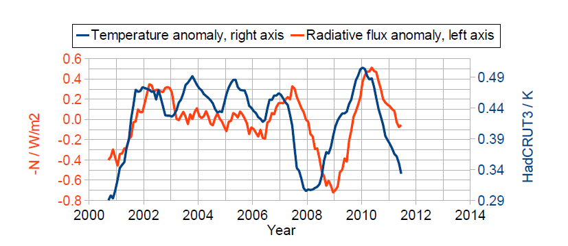
The next figure 6 ( = fig.1 of the paper) shows how the -net radiation and the global surface temperature (all anomalies) changed during the period of investigation:
 fig.6. Variations of -net and global Hadcrut3 temperature anomalies (13 month moving average applied)
Clearly the red curve (-net) lags the temperatures with about 7 months, and the variations are greatest during the 2006-2011 period, which is one of high ENSO indices. Drawing the phase plot with shifting the -net points by 7 months to the right gives the following result (fig. 2b of the paper):
 fig.7 Phase plot of the lag-shifted (-net, temperature) for mid-2006 to mid-2011.
The red line is simply a least square regression line and has a slope of 5.3 +/- 0.6 W/(m2*K); clearly large portions of the phase plot are more or less parallel to the red line. If we assume that the only (major) forcings during that period are those from the natural occurring La Niño and La Niña, the slope of 5.3 would represent the climate sensitivity parameter lambda. As the equilibrium climate sensitivity is often defined versus a doubling of the CO2 concentration from 280 to 560 ppm with a corresponding forcing of 3.71 W/m2, the warming to be expected from such a doubling would be in the interval [3.71/5.9; 3.71/4.7] = [0.63; 0.79 °C], much less than the “consenus” IPPC intervall of [2; 4.5 °C].
Pehr Björnhom must be highly acclaimed for the addendum to his paper, where he gives all the necessary instructions how to obtain the data and make the relevant calculations; this is an exemplary openness and a admirable scientific conduit which all true scientist and researcher should follow. I found a very small glitch in his Scilab script, which was easily corrected and did not have an influence on the calculation.
6. Conclusion
These 3 papers follow similar but not identical lines of reasoning; all suggest a climate sensitivity that is very small and distinctively lower than 1°C. The warming stand-still observed during the last decade (or even 16-18 years) seems to favor that interpretation, as CO2 mixing ratios from 1998 to 2012 increased from approx. 367 to 394 ppm, corresponding to a related change in forcing of 0.4 W/m2 (about 4 times higher than the change in solar TSI from minimum to maximum during a solar cycle) which seems to have no warming effect.
Probably Björnhom’s paper will be heavily criticized as was the case with the 2 other papers; this is a normal scientific procedure if these criticism is valid and done in a civilized manner. In my opinion, the final and definitive answer to the climate sensitivity problem is not yet here.