COVID-19: calculations and curves (1 of x)

 

1. Introduction

With the spread of the new and nasty corona virus modelling and calculations about pandemics and spread of infection spring up about everywhere. Now the interest and the mathematics of handling such a situation are not new, and are a standard subject for all students of differential equations. As an example, let me give an example from a publicity brochure for the Hitachi 200x hybrid analog computer from the 60’s:

(~1967, click here to download the full brochure).

Here is the example problem:

A system of 3 non-linear differential equations is enough to model the situation, and the plotter driven by the analog computer outputs this graph:

A very long time ago, Benjamin Gompertz (1771 – 1865) published a sigmoid-type function that often fits well to the first or all parts of the infection (above for instance the curve Z). The Gompertz function has only 3 parameters and is:

y(t) = a*exp(-b*exp(-c*t)).

When t tends to infinity, exp(-c*t) -> 0  and exp(-b*0) = 1; so when t -> infinity, a becomes an asymptote ( in the curve Z all persons become immune in the long run).

Willis Eschenbach has an excellent article in the Wattsupwiththat blog titled “The Math of Epidemics“, where he applies the Gompertz function to the Covid-19 cases in South Korea, and the fit is excellent:

His article put me on the rails to do the same with the situation in Italy (start of the epidemic is 25 Feb 2020), all relevant data are published live here.

2. Gompertz function and Covid-19 in Italy

This is the Gompertz-function applied to the death cases, as published today 18-March-2020:

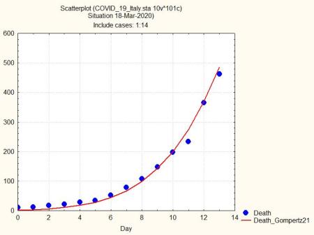
The fit is excellent, and all 3 parameters are statistically significant; the interval between the lower and upper confidence levels is [6741, 45889], and the fraction of (std.error of a)/a has become 35%. The relative errors and the width of the confidence interval will narrow with more data points available. When only few points is all you have, do not make any prediction! The next figure shows the plot from above, extended up to 100 days, and also the same exercise when only 14 and 15 data points were available:

When only 15 or 14 data points are available, the confidence interval becomes ridiculous; it is only for the latest plot with 21 points that all three parameters become significant at the 95% level. So beware to massage your asymptote for any serious meaning, if you have too few data!

 

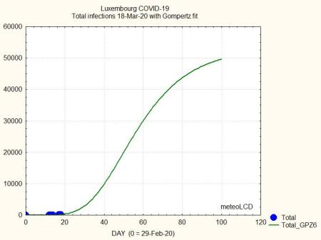
3. The Gompertz curve and Covid-19 in Luxembourg.

Tiny Luxembourg (~675000 inhabitants) only started the epidemic in Feb. 29th. Until today we have only 6 data point for the total infected (up to 203 today) and 2 cases of death. Here what the Gompertz fit looks like for the total infected:

But look at the enormity of the confidence interval! Even if the Gompertz calculation gives near identical results as the observations, all parameters are not significant and one should never see the asymptote in the next graph as an intelligent predictor for the maximum number of infections!

 

(to be continued)